
Terminology
In this section you will find the explanation of the terminology we use.
What is probability distribution?
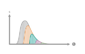
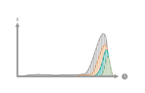
A lead time probability density function (PDF) is a “best fit” curve, that shows the distribution of actual data for lead time from a Kanban system.
Fat-tailed distribution
Poor predictability, potentially high impact from long delays.
Thin-tailed distribution
Good predictability, low impact, shorter delays
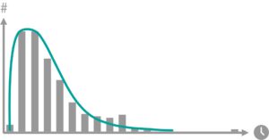
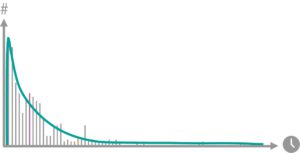
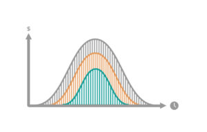
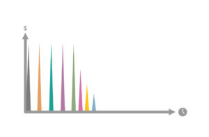
The x-axis shows the number of days of lead time, and the y-axis shows the occurrence of that time within the sample data set (the number of items pulled through the Kanban system).
The example on the left is from an IT Operations group and the one on the right is from a software product development team. It is said to be “fat-tailed”: there is a long visible tail stretching out to the right along the x-axis. Generally speaking, “fat-tailed” is undesirable, risky, and makes planning difficult. The one on the right is said to be “thin-tailed”: there isn’t a long visible tail running off to the right along the x-axis. This naming convention can seem counterintuitive to non-mathematicians. The truth is that mathematically, these tails run to infinity. Hence, if you can see the tail, it must be fat. A thin tail is effectively invisible along the x-axis. These concepts of fat-tailed and thin-tailed lead time distributions are very important and knowing which one you have in your Kanban system makes a vital difference to planning, risk management, and your likelihood of achieving customer satisfaction and being viewed as a trustworthy service provider.
With no data about the probability distribution of the working item we recommend assuming fat-tailed distribution. It is important to remember this simple mantra: “the risk is always in the tail”. Fat-tailed distributions require a different approach to managing risk.
What is lead time?
We define lead time as starting at the mutually agreed commitment point and continuing until an item is ready for delivery. In other words, we start counting lead time from the point when a customer can legitimately expect us to work on it, until we can legitimately expect the customer to take delivery. Any additional waiting on the delivery end is not counted. This definition is unambiguous and works consistently for any workflow and service.
Given Kanban Maturity Model studies we should, however, recognize that this definition works reliably at maturity level 3 and deeper, while at lower maturity levels it is problematic. At lower maturity levels, the commitment point is often ambiguous and at best asynchronous, i.e. the customer/upstream commit a request, before the delivery/downstream service workflow is ready to commit. In this case, of asynchronous commitment, we measure lead time from the 2nd half of the commitment, the point when the delivery workflow pulls the item into WIP. Often in maturity level 2 workflows there isn’t a strong concept of commitment and hence, there is a tendency to measure lead time from the point a work item is submitted. This is legitimate for internal shared services and other similar systems where the work is irrefutable.
The term “lead time” therefore means, “If you know when you need to take delivery, the lead time, is the amount of time you need in advance in order to place an order and expect delivery on or before when you need the item,” or simply, the period of time that commitment must lead delivery.
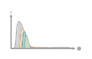
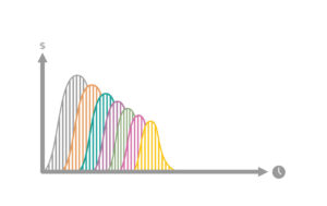
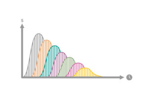
What is value acquisition lifecycle curve?
Acquisition lifecycle curve shows the rate of value acquired over time. The area under the curve is the total value acquired. The length on the x-axis is the lifecycle – the period of the time while the product or service or feature is available and generating benefit.
The graphics show different lifecycle value acquisition curves and how the curve would change if there is a delay in delivery and availability to create value.
1. One-off opportunity with an expiry date
The impulse function implies that there is a one-off opportunity to gain a benefit (make money) and after that opportunity, the chance is gone.
A customer with a remaining annual budget approaches you to spend the money before the new fiscal year. You either take the opportunity before the expiry date or lose the sale.
2. Very front loaded
80 percent of the benefit is realized in the first 20 percent of the lifecycle.
A ski manufacturer issues new models every year in November, and most of the skis are sold in the first three months of what is a one-year lifecycle.
3. Front loaded
80 percent of the benefit is realized in the first 50 percent of the lifecycle.
A bicycle manufacturer, as in previous example, issues new bicycles every year in November–December, but the majority of sales happen in the beginning of the season—in spring—and drop off toward the end of the summer.
4. Bell curve, no catch up
A bell curve with “no catch up” implies that there is a network effect in the marketplace that gives the first mover an advantage that cannot be taken away later.
This network-effect, first-mover advantage is often associated with technology platforms such as operating systems, productivity suites, mobile telephony standards, messaging and communications tools, and social media networking.
5. Bell curve with catch up
A bell curve with catch up has no first-mover advantage, and second and subsequent movers can catch up and even overtake an early market mover.
The first car manufacturer that introduced LED lights in the market had an advantage, and it took one year for a second manufacturer to offer the same technology. Then it took several years for other market players to catch up. Nevertheless, the first player didn’t have a lock-in market effect, and it didn’t affect competitors’ sales.
6. Back loaded
80 percent of the benefit is realized in the last 50 percent of the lifecycle.
A hotel’s Easter marketing campaign starts after the New Year (90–100 days’ lifecycle). Most of the reservations are made in the second half of the lifecycle.
7. Very back loaded
80 percent of the benefit is realized in the last 20 percent of the lifecycle.
A conference organizer offers an event in a local region or metropolitan area aimed at attendees from that geographical region. Unless there is a perceived scarcity of tickets, attendees wait until the last 20 percent of the lifecycle before purchasing a ticket.
8. Constant rate
The constant rate function models the benefit for things such as cost-saving features.
When the product or service is deployed, cost is saved—perhaps workers are made redundant. Consequently, if we had that feature today, we would have the savings tomorrow, and the amount saved is fixed and constant.
9. Bell curve extended, decaying life, decaying loyalty
This models an extended but shortening lifecycle, together with decaying loyalty. These are situations where a delay in releasing a product, feature, or service beyond the desired date has little impact due to customer loyalty, technology lock-in, or monopoly of supply or limited choice in the market. However, long delays cause the lifecycle period to shorten and loyalty to drop off.
Loyal customers will wait for their favorite brand (e.g., mobile phones, laptops, tablets) to release the product with the newest technology (e.g., processor, video chip sets, cameras, etc.). But the delay reduces both the loyalty and the lifecycle of the product because underlying technologies will be replaced in their own independent lifecycle.
10. Bell curve, extended life, decaying loyalty
This models an extended lifecycle, with decaying loyalty over time. These are situations where a delay in releasing a product, feature, or service beyond the desired date has little impact due to customer loyalty, technology lock-in, or monopoly of supply or limited choice in the market.
Microsoft Windows and Apple iPhone/iOS are both examples, but more subtly, so is the next album from a popular rock band such as Depeche Mode or Coldplay. Depeche Mode release albums on a four-year cadence, but were there to be a delay, the loyal fans would wait and still buy the album. However, longer delays eventually cause loyalty to drop off.
11. Last-minute decay
Immediate benefits regardless of the delay, however, last-minute results in a rapid drop-off in realized benefits.
This models a business such as promoting a pop concert for a popular artist, such as Taylor Swift. If the tickets go on sale today, the whole stadium is sold out within hours. If we delay a week or a month, we still sell out. The perception of scarcity means that the sales are immediate regardless of the delay, unless we wait to the last minute without announcing the event.
Select customer expectations
What is that?
What are your customer’s expectations with respect to the desired delivery date?
“Don’t Care”. Are your clients laissez-faire and unconcerned? The date is merely advisory or there isn’t really a specific date, one was simply invented for the purpose of this exercise? Could we say, they don’t mind when it is delivered, so long as it eventually happens? If so, then your customer expectation is “Don’t Care”.
Within SLA/SLE. Is there an SLA/SLE in place with the customer, and hence, if we start an item, there is an expectation that we deliver it within that time? If so, then your customer expectation is “Within SLA/SLE”.
Deadline. Does the desired delivery date come with a demand of a deadline? The deadline may be real as in a fixed date for an external event or something season in nature. Or it may simply be an instrument of a low trust environment – the deadline is being used to squeeze us, as a stressor to drive action, or somehow to hold us accountable, in an otherwise low trust culture. Regardless of the reason if the customer demands a deadline then we should account for it.
“Zero tolerance”. When there is a genuinely high cost of delay beyond the desired delivery date, the customer may have “zero tolerance”. This is a more extreme form of deadline – when there is zero tolerance for delay, everyone will understand the consequences and impact to our business of a failure to meet the deadline. We are likely to sacrifice many other work items in order to achieve the date.
ASAP. Finally, the customer expectation may be “as soon as possible” (ASAP) in which case, if we choose to do the work, we will need to expedite the request.
What is lifecycle period?
When a work item is delivered to the customer how long does the benefit live.
Tell me more about my result
Fixed Date. At a date in the relatively near future, within twice the range of the lead time distribution, we expect a step function impact (or a sloping s-curve function very close to a step function) on a known and very specific day, typical of seasonal demand, or specific named events (such as sports tournaments, or public holidays)
Standard. The cost of delay rises over a period defined by the range of the lead time and the range of the lifecycle, initially in a convex pattern and eventually becoming concave. The shape is an s-curve over a medium to long period of time;
Intangible – named for the fact that the cost of delay is intangible or insignificant for a period longer than 1 to 2 cycles of the lead time range. While we model the Intangible class of service as having a convex function shape, we learned that these are in fact, also s-curve functions. Intangible class of service work is commonly observed with platform upgrades, incorporating new components or technologies into an existing design, or redesigning, reworking or generally, system maintenance on a product or service, or its design or source code.
Class of Service – how do we treat this relative to other requests?
Priority can mean whether something is selected (or chosen) and hence “given priority.” It can also imply the sequencing, order or queuing discipline in which a set of items are to be worked. Or priority can imply when something should be scheduled: now; later and if so when; or not at all. Or it can imply how something is treated once it is in the system: its class of service.
Triage tables are designed to help with the last two of the four meanings for priority. They will help you schedule work and determine the class of service to be applied to a piece of work given its scheduled start date.
What do you mean by cost of delay?
Cost of Delay. Delay means we make less value from an opportunity. Cost of Delay attempts to approximate the value lost due to delay. The cost of delay can be modeled as a curve as it accumulates over time. If the shape of the curve spikes early, then cost of delay risk is significant.